IṢẸ́ ỌNÀ
ẸWÀ ÀTI ÌLERA
IṢẸ́ ỌWỌ́
ÀṢÀ ÀTI ÌTÀN
ÌṢERÉ
ÀYÍKÁ
OÚNJẸ ÀTI OHUN MÍMU
REVERSE ENGINEERING
SÁYẸ́ǸSÌ
ERÉ ÌDÁRAYÁ
ÌMỌ̀-Ẹ̀RỌ
ÀWỌN OHUN WÍWỌ̀


PID and Ziegler-Nichols Tuning
The three terms answer three different questions about the same error. Proportional asks how wrong am I - it acts at once and always leaves some error behind, because zero error would mean zero output. Integral asks how long have I been wrong - it keeps pushing until the error is gone, and it is the only cure for the droop Maxwell described in 1868. Derivative asks how fast is it changing - it is Sperry's rate term, damping the loop.
None of that was new in 1942. What John Ziegler and Nathaniel Nichols contributed at Taylor Instrument was a way to SET them without knowing anything about the process. Turn the proportional gain up, with the other two at zero, until the plant oscillates steadily; call that gain Ku and time the swings to get Tu. Then read six numbers off a table: for a full three-term controller, Kp is 0.6 Ku, the integral time is Tu over 2 and the derivative time is Tu over 8. A plant engineer with a stopwatch and no model could tune a loop in an afternoon, and eighty years later most of the loops running in the physical world were still set that way.
It is worth knowing what the table is aiming at, because it is aggressive. Ziegler and Nichols targeted quarter-amplitude damping - each swing a quarter of the one before - which recovers from an upset quickly and overshoots hard on the way. That is right for a process that must shrug off disturbances and quite wrong wherever overshoot is expensive, so every handbook since has published gentler variants of the same six numbers.
Two things the equation does not mention will decide whether your loop works. The derivative term differentiates the sensor's noise as happily as the signal, and the integral term keeps accumulating while the heater is already flat out - which is why a controller without anti-windup is not a PID controller but a PID controller with a fault.
Àárín
4 hours
Ìlànà
1
1
A plant with a real dead time
A plant with a real dead time
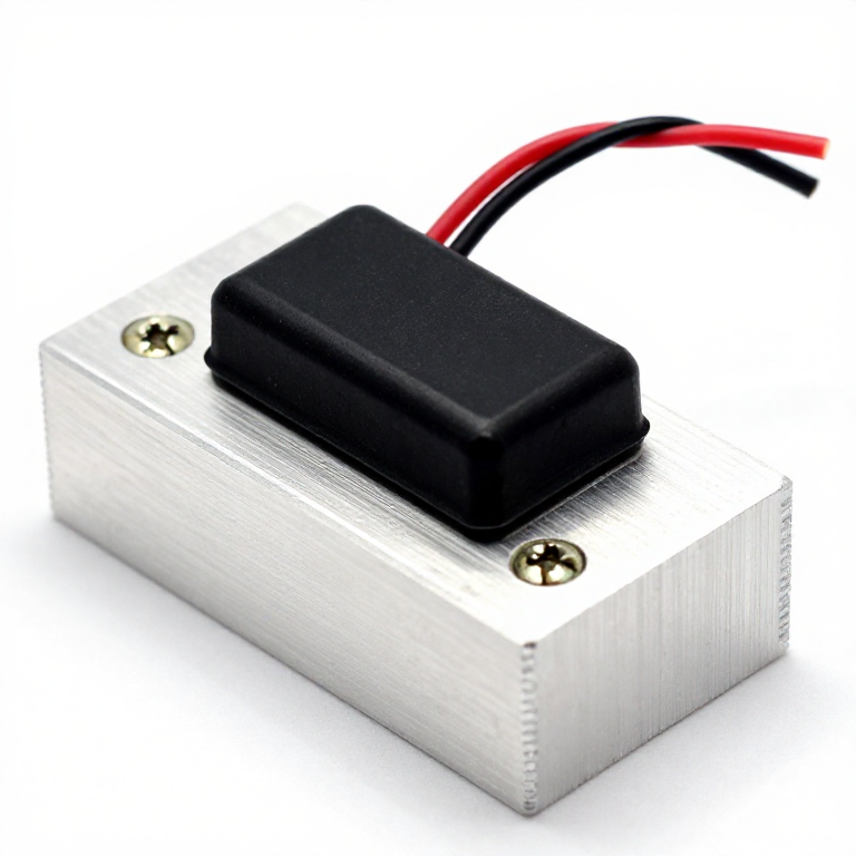
Bolt a 10 W power resistor to one end of a short aluminium bar and press the thermistor into a hole at the other end, with a smear of thermal paste in both.
That gap is the point. Switch the heater on and time how long it takes the thermistor to move at all - several seconds of pure dead time, which is what makes this loop hard and what a bare thermistor on the resistor would hide.
Àwọn ohun èlò fún ìgbésẹ̀ yìí:
 Ọ̀pá pẹlẹbẹ ti aluminium150 mm
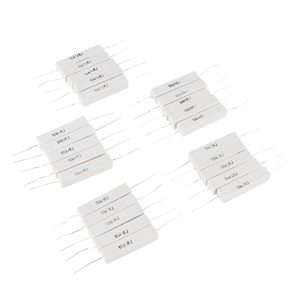 Power Resistor Kit - 10W (25 pack)1 ohun èlò
 Ìkójọpọ̀ thermistor NTC1 ohun èlò
 Ìdàpọ̀ ooru (Arctic Silver)1 tube
Àwọn irinṣẹ́ tí a nílò:
 Ẹ̀rọ Ìlùkòkò Aláìlókùn
 Aago Ìdúró
 Òṣùwọ̀n Oníṣirò Díjítà Ìpele Yàrá Ìwádìí
 Ìpèsè Agbára Tábìlì
2
2
The controller, with the two lines nobody mentions
The controller, with the two lines nobody mentions
One constant selects on/off, P, PI or PID; the gains come from Ku and Tu through the Ziegler-Nichols table.
Measure Ku and Tu on YOUR block first - raise Kp with the other terms at zero until the temperature swings steadily, then time it. Run all four modes and you have the notebook's table in your own hardware.
pid_heater.inocpp
Àwọn ohun èlò fún ìgbésẹ̀ yìí:
 MOSFET onípa-ọ̀nà N ti IRF540N1 àkópọ̀
 Àkójọ Rẹsístà 1/4 W1 ohun èlò
 Ìdìpọ̀ okùn Dupont (akọ-abo)1 ìtò
Àwọn irinṣẹ́ tí a nílò:
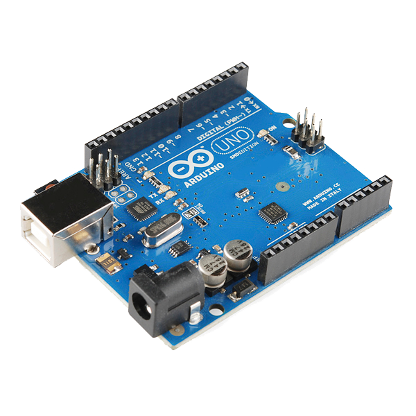 Arduino Uno R3 SMD
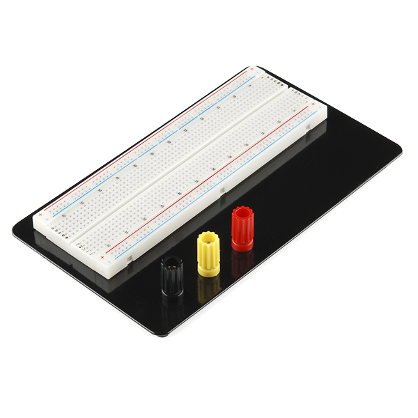 Breadboard - Classic
 Kọ̀ǹpútà TábìlìÌpèsè Agbára Tábìlì
3
3
Ku, Tu, the table, and four controllers compared
Ku, Tu, the table, and four controllers compared
Ń ṣí ìwé Jupyter…
Àwọn irinṣẹ́ tí a nílò:
Kọ̀ǹpútà Tábìlì4
4
Compendium: the other method, and what Ku costs to find
Compendium: the other method, and what Ku costs to find
Ziegler and Nichols published two methods and the one everybody quotes is the harder one to use. Finding Ku means deliberately driving a live process into sustained oscillation, which on a chemical plant, a furnace or anything with a safety case is not a reasonable thing to do. Their open-loop method avoids it entirely: put a step into the plant with the controller off, draw a tangent at the steepest point of the response curve, and read off the apparent dead time L and the slope R. The gains follow from those two numbers alone - for a PID, Kp is 1.2 over R L, the integral time is 2 L and the derivative time is 0.5 L - and the plant is never asked to misbehave.
Both methods are really estimating the same thing, which is how much phase the plant spends before its gain runs out. That is Nyquist's question from ten years earlier, and the ultimate-sensitivity experiment measures the answer directly: at the point of steady oscillation the loop gain is exactly one and the phase exactly minus 180 degrees, so Ku and Tu ARE the coordinates of the critical point. The 1942 table is Nyquist's criterion reformulated as something you can do with a knob and a stopwatch, which is why it spread through industries that never read the 1932 paper.
Àwọn ohun-èlò
7- 150 mmÀyè
- 1 ohun èlò$5.61
- 1 ohun èlòÀyè
- Àyè
- 1 àkópọ̀Àyè
- 1 ohun èlòÀyè
- Àyè
Àwọn irinṣẹ́ tó nílò
7- 1 vendor sell this, none ship to you yetÀyè
- Àyè
- Arduino Uno R3 SMDìdá 10%$26.68
- Breadboard - Classicìdá 10%$9.37
Àpapọ̀ Ìfojúsùn
Ohun tí ẹni tó ṣe é rà. Àwọn ohun èlò tí kò ní iye owó ni o máa rà níbi tí o bá ti rà á.
Blueprint tó jọra
Àwọn blueprint wọ̀nyí pín ìmọ̀ — ọ̀nà, ohun-èlò tàbí ìlànà


CC0 Àgbègbè Gbogbogbò
Blueprint yìí ti jáde lábẹ́ CC0. O lè ṣe àdàkọ, yí padà, pín, àti lò láìsí ìyọ̀ǹda.
Ṣàtìlẹ́yìn Olùṣẹ́dá nípa rírà àwọn ọjà nipasẹ̀ Blueprint wọn Ẹ̀san Olùṣẹ́dá tí àwọn Olùtajà gbé kalẹ̀, tàbí ṣẹ̀dá àtúnṣe tuntun ti Blueprint yìí kí o sì fi sínú Blueprint rẹ gẹ́gẹ́ bí ìsopọ̀ láti pín owó-wíwọlé.