МИСТЕЦТВО
КРАСА ТА ЗДОРОВ'Я
РЕМЕСЛО
КУЛЬТУРА ТА ІСТОРІЯ
РОЗВАГИ
СЕРЕДОВИЩЕ
ЇЖА ТА НАПІЇ
ЗБОРНА ІНЖЕНЕРІЯ
НАУК
СПОРТ
ТЕХНОЛОГІЯ
НОСИМО


Hounsfield Computed Tomography
Every earlier blueprint in this batch answers the same question - what can I throw away so that what remains is legible? The grid discards photons from the wrong direction. Planigraphy discards everything not at one height. Subtraction discards everything that did not change. Each one destroys real information to make a picture a human can read.
**Godfrey Hounsfield asked a different question: what if you keep all of it and SOLVE for the object?**
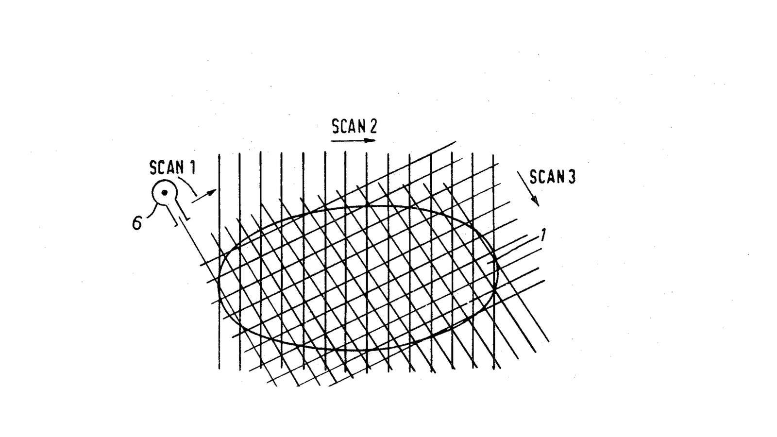
A radiograph from one direction gives you, for every ray, the total absorption along that line. One equation, many unknowns - hopeless. But take views from many angles and every point in the slice is crossed by many different rays, each contributing to a different sum. Now you have thousands of equations in thousands of unknowns, and that is not hopeless at all. It is arithmetic.
**US 3,778,614**, "Method and apparatus for measuring x- or γ-radiation absorption or transmission at plural angles and analyzing the data", Godfrey Newbold Hounsfield, assigned to EMI, filed 27. December 1971 and granted 11. December 1973. The claim describes transmitting radiation through many paths in a planar slice at varying angles and then using **"a process of successive approximations"** to calculate the absorption of each element of a matrix. That phrase is worth noticing: Hounsfield's own method was iterative, guessing and correcting, not the filtered back-projection that machines settled on soon after.
The mathematics was not new. Recovering a function from its projections had been solved decades earlier by Johann Radon, as pure mathematics, with no machine and no computer to use it on. Allan Cormack worked out the medical application independently in the 1960s, and shared the 1979 Nobel Prize in Physiology or Medicine with Hounsfield for it.
**What CT actually bought.** Soft tissues differ in absorption by a per cent or two. On a radiograph that difference is buried under everything in front of and behind them; no grid, no tomogram and no subtraction recovers it. Solving for each element separately does. For the first time you could see grey matter distinct from white matter, and a clot distinct from the brain around it.
**You will build a scanner and reconstruct a slice with it.** Not with X-rays - with light, a turntable and a sensor - and the notebook does real filtered back-projection on your data. The algorithm does not care what did the shining.
Середній
4 hours
Інструкції
1
1
Build the gantry: turn the object, not the source
Build the gantry: turn the object, not the source
Hounsfield rotated the source and detector around the patient because patients do not like being spun. You have no such constraint, and turning the object is far easier to build accurately.
Mount a small turntable - a stepper motor with a disc on it, or a manual rotary stage with degree markings - and fix a light source and a sensor on opposite sides, aligned so the beam passes through the centre of rotation. Getting that alignment right matters more than anything else in the build: if the axis of rotation is not on the beam line, every view is offset from every other and the reconstruction smears in a circle.
**Check it before going further.** Put a thin pin upright at the centre of rotation and turn the table a full revolution. If the pin's shadow stays in the same place on the detector throughout, the axis is aligned. If it swings, adjust and repeat. Ten minutes here saves an evening later.
A stepper with a driver board gives you repeatable angles, which is worth having; a printed protractor and a steady hand is entirely adequate for a first scan.
Матеріали для цього кроку:
 Кроковий двигун (NEMA 17)1 штука
 Лист фанери1 штука
 Гвинт із циліндричною головкою та внутрішнім шестигранником6 штук
 Шестигранна гайка6 штук
 Кульковий підшипник1 штука
Необхідні інструменти ({count})
 Акумуляторний дриль
 Цифровий штангенциркуль 6 дюймів
 Лінійка
 Транспортир
 Набір шестигранних ключів
2
2
One view: a single line of measurements
One view: a single line of measurements
A view is the transmission along each of many parallel rays through the object at one angle. Two ways to collect it, and the second is much faster.
**The honest way, one ray at a time.** Put a narrow slit in front of the source, a photodiode behind the object, and translate the whole assembly across in steps, reading the sensor at each. That is precisely what the first EMI scanner did - translate, rotate, translate, rotate - and it is why early scans took minutes per slice.
**The fast way, all rays at once.** Photograph the backlit object with a camera and take ONE ROW of pixels from the image. That row is a complete view: every pixel in it is a different parallel ray. A camera is a detector array, which is what every scanner after the first generation used.
Either way, convert to absorption before you do anything else. The detector measures transmitted intensity, and absorption along a ray is the **negative logarithm** of transmitted over incident. This is the same logarithm as the subtraction blueprint, for the same reason: attenuation multiplies, and you need it to add before you can solve linear equations with it.
Матеріали для цього кроку:
 Фотодіод (BPW34)1 штука
 Акриловий лист1 штука
Необхідні інструменти ({count})
 Цифрова фотокамера
 Світлодіодний ліхтар для огляду
 Настільний комп'ютер
 Штатив (карбон, кульова голова)
3
3
Collect a sinogram
Collect a sinogram
Choose a phantom you know the truth about: a block of clear acrylic with holes drilled in it, some filled with water and one with a short length of steel bar, is ideal. You want several materials whose real positions you can measure with a caliper afterwards.
Take a view every two degrees through 180 degrees - ninety views. **One hundred and eighty is enough, not three hundred and sixty**: a ray through the object from one side measures the same total absorption as the same ray from the other side, so the second half of a full turn is redundant.
Stack the views into an array, one row per angle. That array is the sinogram, and it is worth looking at: a single point in the object traces a sine wave down it, which is where the name comes from and which is the quickest way to spot a misaligned axis - the sine should be centred, not drifting.
**This is everything a CT scanner physically collects.** There is no image in it anywhere. Everything after this point is arithmetic.
Матеріали для цього кроку:
Акриловий лист1 штука Пруток із низьковуглецевої сталі1 штука
 Дистильована вода100 мл
Необхідні інструменти ({count})
Настільний комп'ютерЦифровий штангенциркуль 6 дюймівТранспортир4
4
Reconstruct, and then compare with the caliper
Reconstruct, and then compare with the caliper
Run your sinogram through the notebook step. Do it twice: once with plain back-projection and once filtered.
Plain back-projection gives a recognisable shape in a thick haze. That haze is not noise and no amount of averaging removes it - it is a systematic consequence of smearing every view across the whole plane, which counts the centre far more often than the edges.
Filtered back-projection sharpens each view with a ramp filter before smearing it, which cancels that over-counting exactly. The difference is not subtle; it is the difference between an idea and an instrument.
**Then do the thing that makes it a measurement.** Take your reconstruction, find the steel rod in it, and measure its diameter and position in pixels. Convert to millimetres using a known dimension of the phantom. Now take the caliper to the real phantom.
Write the two columns side by side. If they agree to a millimetre or two you have not made a picture of the inside of an object - you have MEASURED the inside of an object without opening it, which is a different and much larger claim.
Необхідні інструменти ({count})
Настільний комп'ютерЦифровий штангенциркуль 6 дюймів5
5
Filtered back-projection, from first principles
Filtered back-projection, from first principles
Завантаження блокнота Jupyter…
6
6
When the slice will not come out
When the slice will not come out
The two commonest failures look nothing alike and are both about sampling. Work down in order.
Flow
Loading...
7
7
Compendium: Hounsfield units, dose, and the return of the guess
Compendium: Hounsfield units, dose, and the return of the guess
**The Hounsfield unit.** Absorption is reported on a scale fixed by two definitions: water is 0 HU and air is −1000 HU. Everything else falls where it falls - fat slightly negative, soft tissues a few tens positive, bone in the hundreds to thousands - and the displayed range runs from about −1024 to +3071. Because the scale is anchored to materials rather than to a machine, a number means the same thing on any scanner anywhere, which is why radiologists can quote it as a diagnostic finding.
**Windowing, which follows from that.** The full scale is four thousand values and a screen shows a few hundred greys, so the radiologist selects a window - a centre and a width - and everything outside it is pure black or pure white. The same scan is read several times with different windows for lung, soft tissue and bone. Nothing is discarded; the data holds all of it, and the window is only how a human looks at it.
**Dose, honestly.** CT gives far more information than a radiograph and delivers considerably more dose than one. It is the largest single contributor to medical radiation exposure in most countries, and the justification for each scan is a real clinical decision rather than a formality. This is the one modality in the batch where more use is not automatically better.
**Spiral, multi-slice, and speed.** Move the patient continuously while the tube rotates and the beam traces a helix - which removes the stop-start of slice-by-slice scanning and makes a whole chest possible in one breath-hold. Add rows of detectors and you acquire many slices per rotation. A modern scan takes seconds where the first took a coffee break per slice.
**And Hounsfield's own method came back.** Filtered back-projection displaced successive approximation for decades because it was fast and computers were slow. Modern scanners increasingly use iterative reconstruction again - guess an object, forward-project it, compare with what was measured, correct, repeat - because it handles noise far better and therefore permits a LOWER dose for the same image. The patent's own phrase, "a process of successive approximations", describes what the best scanners now do, fifty years after it was too slow to use.
Матеріали
9- 1 штукаЗаповнювач
- 1 штукаЗаповнювач
- Заповнювач
- 6 штукЗаповнювач
- Заповнювач
- 1 штукаЗаповнювач
- 1 штукаЗаповнювач
- Заповнювач
- 100 млЗаповнювач
Необхідні інструменти
9- 1 vendor sell this, none ship to you yetЗаповнювач
- Заповнювач
- Заповнювач
- Заповнювач
- Заповнювач
- Заповнювач
- Заповнювач
- Заповнювач
- Заповнювач
Пов'язані креслення
Ці креслення діляться знаннями — техніки, матеріали або принципи


CC0 Суспільне надбання
Це креслення випущено під ліцензією CC0. Ви можете вільно копіювати, змінювати, поширювати та використовувати цю роботу для будь-яких цілей без запиту дозволу.
Підтримайте мейкера, купуючи продукти через його креслення, де він отримує Комісію мейкера встановлену вендорами, або створіть нову ітерацію цього креслення та включіть його як зв'язок у власне креслення для розподілу доходу.